Workshop 2 - Animal model

Sylvain SCHMITT

2019-12-18

Introduction

Setup

rm(list = ls()) ; gc()

##          used (Mb) gc trigger (Mb) max used (Mb)
## Ncells 460922 24.7     996122 53.2   641594 34.3
## Vcells 883665  6.8    8388608 64.0  1752615 13.4

library(knitr)
library(tidyverse)
library(rstan)
library(bayesplot)
theme_set(bayesplot::theme_default())
options(mc.cores = parallel::detectCores())
rstan_options(auto_write = T)
opts_chunk$set(echo = T, eval = T, cache = T, fig.height = 5)

A Phenotype

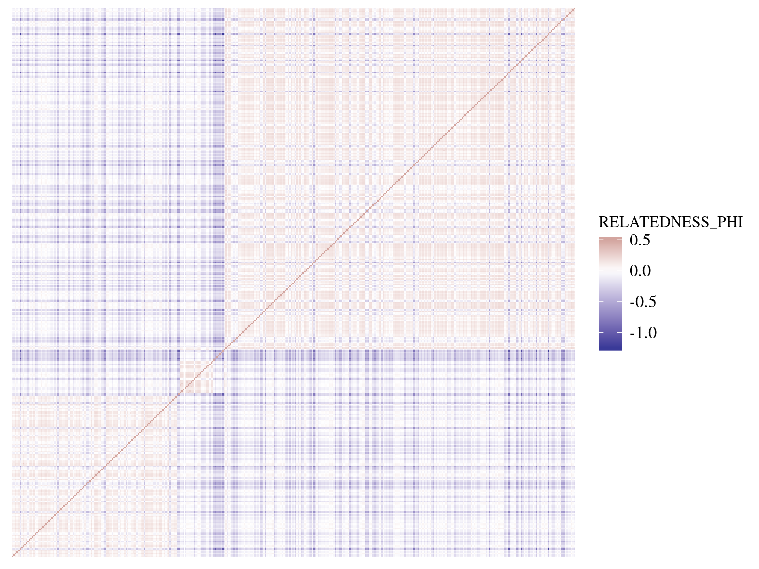
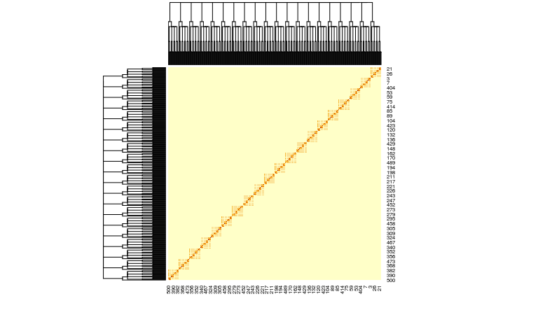
A Kinship matrix

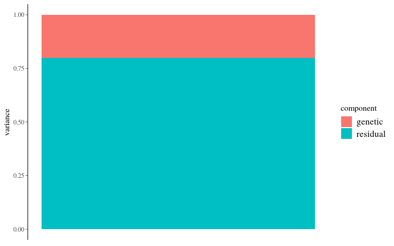
Genetic variance

How much of my phenotype is explained by genetic ?

Maths

Animal model

\[y \sim \mathcal N(\mu + u, \sigma_E)\]

\[u \sim \mathcal{MVN}_N(0, \sigma_GK)\]

\[\sigma_P = \sigma_G + \sigma_E\]

\(y\) vector of \(N\) individuals phenotypes
\(\sigma_P\) the phenotypic variance
\(\mu\) the mean phenotype
\(K\) matrix of \(N\times N\) between-individuals kinship
\(u\) vector of \(N\) random effects of individual kinship
\(\sigma_G\) phenotypic variance explained by genetic
\(\sigma_E\) residual phenotypic variance unexplained by genetic

Multivaraite normal distribution

Multivaraite normal - PDF

\(\mathcal{MVN}_N(\mu,\Sigma)\)

If \(\Sigma\) is positive-definite, MVN is “non-degenerate”

\[f(x\mid\mu,\Sigma) = \frac{exp(-\frac 12 (x-\mu)^T\Sigma^{-1}(x-\mu))}{\sqrt{(2\pi)^kdet(\Sigma)}}\]

Multivariate normal - Normal random vector

\[X \sim \mathcal{MVN}(\mu,\Sigma) \iff\]

\[\exists \mu \in \mathbb R^k, A\in\mathbb R^{k\times l}\]

\[\mid X = AZ+\mu ~for~Z_n \sim \mathcal N(0,1), i.i.d\]

\[resulting~in~\Sigma=AA^T\]

Multivariate normal - Cholesky decomposition

If \(\Sigma\) is positive-definite

\(\Sigma=AA^T\)

And \(A\) is the Cholesky decomposition of \(\Sigma\)

Cholesky decomposition is implemented in stan !

Back to the Animal model

\[X \sim \mathcal{MVN}(\mu,\Sigma) \iff X = AZ+\mu\mid Z_n \sim \mathcal N(0,1), i.i.d\]

\[u \sim \mathcal{MVN}_N(0, \sigma_GK) \iff \sigma_GA\tilde u \mid\tilde u \sim\mathcal N(0,1)\]

Resulting in:

\[y \sim \mathcal N(\mu + \sigma_GA\tilde u, \sigma_E)\]

\[\tilde u \sim \mathcal{N}_N(0, 1)\]

\[\sigma_P = \sigma_G + \sigma_E\]

with A the Cholesky decomposition of K

Back to the linear model

What about other informations on the individuals ?

\[\mu = \beta_0+\beta_1x_1+..+\beta_qx_q\]

\[\mu = \begin{bmatrix} \beta_0 \\ \beta_1 \\ ... \\ \beta_q \end{bmatrix} [1,x_1,...,x_q] = \beta X\]

\[y \sim \mathcal N(X \beta + u, \sigma_E)\]

To go further

Mathematically the Animal model is the basis of other genomic models including genomic structure throught genetic markers (i.e. SNPs). For instance Linear Mixed Models (LMM), used for major effet detection, or Bayesian Sparse Linear Model (BSLMM), used for polygenic structure inference, are based on the Animal model structure.

Linear Mixed Models - LMM

\[y \sim \mathcal N(\mu + x\beta + u, \sigma_E)\]

\[u \sim \mathcal{MVN}_N(0, \sigma_GK)\]

\[\sigma_P = \sigma_G + \sigma_E\]

with \(x\) one genetic marker and \(\beta\) its effect size on the phenotype

Basyesian Sparse Linear Mixed Models - BSLMM

\[y \sim \mathcal N(\mu + X\tilde \beta + u, \sigma_E)\]

\[u \sim \mathcal{MVN}_N(0, \sigma_bK)\]

\[\tilde \beta \sim \pi\mathcal{N}(0, \sigma_a) + (1-\pi)\delta_0\]

\[\sigma_P = \sigma_a + \sigma_b + \sigma_E\]

with \(X\) the matrix of genetic markers and \(\tilde \beta\) their sparse effects on the phenotype

Stan Univariate

Acknowledgements

Diogo Melo a Brazilian reasearcher from Sao Paulo who originally developed the stan code after a discussion on the stan forum

Data 1

\(y\) vector of \(N\) individuals phenotypes
\(K\) matrix of \(N\times N\) between-individuals kinship

data {
  int<lower=0>  N ; // # of individuals
  real Y[N] ; // phenotype
  cov_matrix[N] K ; // kinship covariance matrix
}

Data 2

\(y\) vector of \(N\) individuals phenotypes
\(K\) matrix of \(N\times N\) between-individuals kinship
\(X\) matrix of \(N\times J\) covariates

data {
  int<lower=0>  N ; // # of individuals
  int<lower=0>  J ; // # of covariates + 1 (intercept)  
  real Y[N] ; // phenotype
  matrix[N,J] X ; // covariates
  cov_matrix[N] K ; // kinship covariance matrix
}

Transformed data

\(\sigma_P\) the phenotypic variance
\(u \sim \mathcal{MVN}_N(0, \sigma_GK) \iff \sigma_GA\tilde u \mid\tilde u \sim\mathcal N(0,1)\)

transformed data{
  matrix[N, N] A ; // cholesky-decomposed kinship
  real<lower=0> sigma ; // phenotypic variance
  A = cholesky_decompose(K) ;
  sigma = sd(Y) * sd(Y) ;
}

Parameters 1

\[y \sim \mathcal N(\mu + \sigma_GA\tilde u, \sigma_E)\]

parameters {
  vector[N]  u_tilde ; // random effects / breeding values
  real mu ; // intercept
  simplex[2] part ; // variance partition
}

Parameters 2

\[y \sim \mathcal N(\beta X + \sigma_GA\tilde u, \sigma_E)\]

parameters {
  vector[N]  u_tilde ; // random effects / breeding values
  vector[J] beta; // fixed effects
  simplex[2] part ; // variance partition
}

Model 1

\[u \sim \mathcal{MVN}_N(0, \sigma_GK) \iff \sigma_GA\tilde u \mid\tilde u \sim\mathcal N(0,1)\]

\[y \sim \mathcal N(\mu + u, \sigma_E)\]

\[u \sim \mathcal{MVN}_N(0, \sigma_GK)\]

model {
    vector[N] u ;
    
    u_tilde ~ normal(0, 1) ; // priors
    mu ~ normal(0, 1) ;
    
    u = sqrt(sigma*part[1])*(A * u_tilde) ;

    Y ~ normal(mu + u, sqrt(sigma*part[2]));
}

Model 1 bis

\[y \sim \mathcal N(\mu + \sigma_GA\tilde u, \sigma_E)\]

\[\tilde u \sim \mathcal{N}_N(0, 1)\]

model {
    u_tilde ~ normal(0, 1) ; // priors
    mu ~ normal(0, 1) ;
    Y ~ normal(mu + sqrt(sigma*part[1])*(A * u_tilde), sqrt(sigma*part[2]));
}

Model 2

\[u \sim \mathcal{MVN}_N(0, \sigma_GK) \iff \sigma_GA\tilde u \mid\tilde u \sim\mathcal N(0,1)\]

\[y \sim \mathcal N(\beta X + u, \sigma_E)\]

\[u \sim \mathcal{MVN}_N(0, \sigma_GK)\]

model {
    vector[N] u ;
    vector[N] mu;
    
    u_tilde ~ normal(0, 1) ; // priors
    to_vector(beta) ~ normal(0, 1) ;

    u = sqrt(sigma*part[1])*(A * u_tilde) ;
    for(n in 1:N)
       mu[n] = beta * X[n] + a[n] ;

    Y ~ normal(mu, sqrt(sigma*part[2])) ;
}

Model 2 bis

\[y \sim \mathcal N(X\beta + \sigma_GA\tilde u, \sigma_E)\]

\[\tilde u \sim \mathcal{N}_N(0, 1)\]

model {
    u_tilde ~ normal(0, 1) ; // priors
    beta ~ normal(0, 1) ;
   Y ~ normal(X*beta + sqrt(sigma*part[1])*(A * u_tilde), sqrt(sigma*part[2])) ;
}

Generated quantities

\[\sigma_P = \sigma_G + \sigma_E\]

generated quantities{
  real sigmaE ; // residual variation
  real sigmaG ; // genetic variation
  sigmaE = sigma*part[2] ;
  sigmaG = sigma*part[1] ;
}

Full

data {
  int<lower=0>  N ; // # of individuals
  real Y[N] ; // phenotype
  cov_matrix[N] K ; // kinship covariance matrix
}
transformed data{
  matrix[N, N] A ; // cholesky-decomposed kinship
  real<lower=0> sigma ; // phenotypic variance
  A = cholesky_decompose(K) ;
  sigma = sd(Y) * sd(Y) ;
}
parameters {
  vector[N]  u_tilde ; // random effects / breeding values
  real mu ; // intercept
  simplex[2] part ; // variance partition
}
model {
    u_tilde ~ normal(0, 1) ; // priors
    mu ~ normal(0, 1) ;
    Y ~ normal(mu + sqrt(sigma*part[1])*(A * u_tilde), sqrt(sigma*part[2]));
}
generated quantities{
  real sigmaE ; // residual variation
  real sigmaG ; // genetic variation
  sigmaE = sigma*part[2] ;
  sigmaG = sigma*part[1] ;
}

R Univariate 1

Variances

h2 <- 0.25 # heritability
sigmaP <-  1 # phenotypic variance (reduced)
sigmaG <- h2 * sigmaP  # genetic variance
sigmaE <- (1 - h2) * sigmaP # residual variance

Variances

Kinship

ped <- read.table("https://raw.githubusercontent.com/diogro/QGcourse/master/tutorials/volesPED.txt", header = T)
inv.phylo <- MCMCglmm::inverseA(ped, scale = TRUE)
K <- solve(inv.phylo$Ainv)
K <- (K + t(K))/2
rownames(K) <- rownames(inv.phylo$Ainv)
K[K < 1e-10] = 0  # Not always exactly positive-definite

Kinship

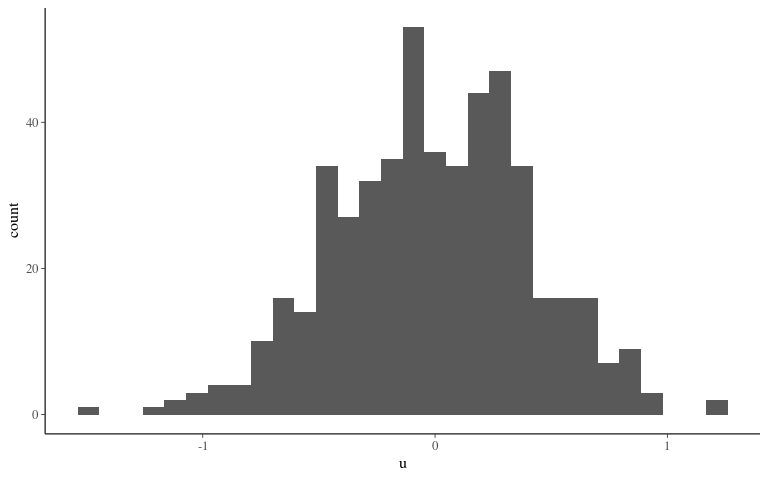
Breeding values

u <- t(mvtnorm::rmvnorm(1, sigma = sigmaG*as.matrix(K)))

Breeding values

Intercept

mu <- rnorm(1)
mu

## [1] -1.00489

Noise

e <- rnorm(nrow(u), sd = sqrt(sigmaE))

Noise

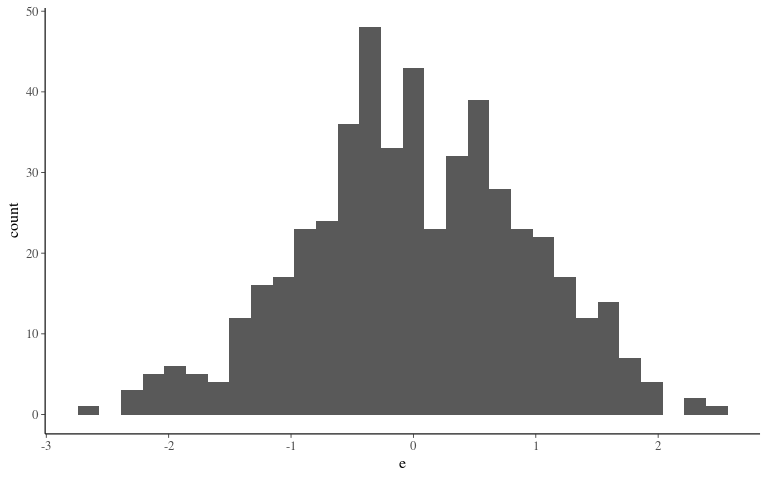
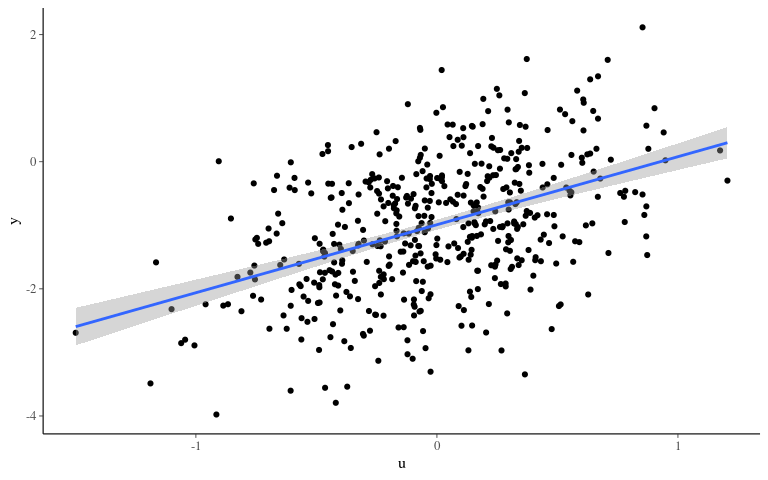
Phenotype

y <- mu + u + e

Phenotype

Inference 1

AnimalUnivariate1 <- stan_model("Animal_models/AnimalUnivariate1bis.stan") 
fitUnivariate1 <- sampling(AnimalUnivariate1, data = list(N = nrow(y), Y = as.vector(y), K = as.matrix(K)), chains = 2, save_warmup = F)
save(fitUnivariate1, file = "Animal_save/univariate1.Rdata")

Convergence 1

## Registered S3 method overwritten by 'xts':
##   method     from
##   as.zoo.xts zoo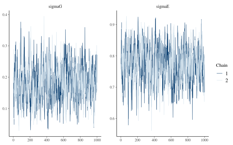

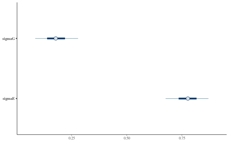
Posteriors 1

R Univariate 2

Covariates

beta <- matrix(c(rnorm(1), rnorm(1)), 2, 1, byrow = TRUE)
rownames(beta) <- c("Intercept", "age")
X <- cbind(rep(1, nrow(u)), rnorm(nrow(u), 5, 3))

Covariates

ggplot(data.frame(age = X[,2]), aes(age)) + geom_histogram()

## `stat_bin()` using `bins = 30`. Pick better value with `binwidth`.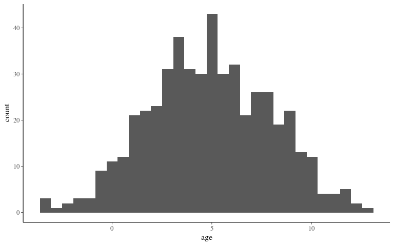

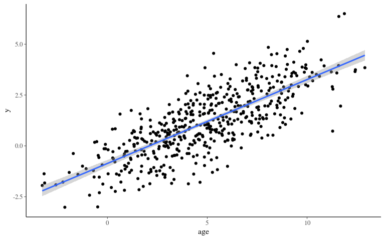
Phenotype 2

y <- X %*% beta + u + e

Phenotype 2

Inference 2

AnimalUnivariate2 <- stan_model("Animal_models/AnimalUnivariate2bis.stan") 
fitUnivariate2 <- sampling(AnimalUnivariate2, data = list(N = nrow(y), J = ncol(X), Y = as.vector(y), X = X, K = as.matrix(K)), chains = 2, save_warmup = F)
save(fitUnivariate2, file = "Animal_save/univariate2.Rdata")

Convergence 2

## Registered S3 method overwritten by 'xts':
##   method     from
##   as.zoo.xts zoo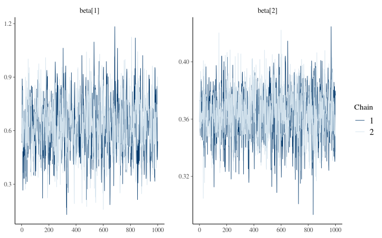

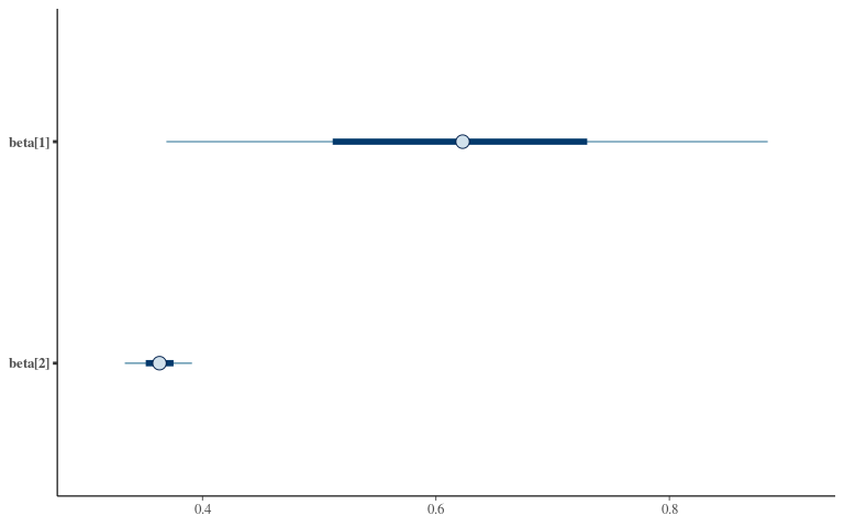
Posteriors 2

## Registered S3 method overwritten by 'xts':
##   method     from
##   as.zoo.xts zoo