Workshop 7 - Dirichlet Multinomial
Sylvain SCHMITT
2020-10-06
Introduction
Setup
##          used (Mb) gc trigger (Mb) max used (Mb)
## Ncells 461322 24.7     997401 53.3   641322 34.3
## Vcells 885270 6.8 8388608 64.0 1753819 13.4Some categorical observation
Distributions.
Mathematics
Dirichlet

Dirichlet - Distribution
Continuous multivariate probability ditribution
Multivariate generalization of beta the distribution
Conjugate of catgorical and multinomial distributions
Dirichlet - Definition
Parameters: categories \(K \geq 2\) and concentrations \(\alpha_1,...,\alpha_K|\alpha_i>0\)
Support: \(x_1,...,x_K|x\in(0,1),\sum_{i=1}^Kx_i=1\)
PDF: \(\frac{1}{B(\alpha)}\Pi_{i=1}^Kx_i^{\alpha_{i-1}}|B(\alpha)=\frac{\Pi_{i=1}^K\Gamma(\alpha_i)}{\Gamma(\sum_{i=1}^K\alpha_i)}\)
Dirichlet - Example

Multinomial - Distribution
Parameters: number of trials \(n > 0\) and event probabilities \(p_1,...,p_K|\sum p_i=1\)
Support: \(x_i\in\{0,..,n\}|i\in\{1,..,k\},\sum x_i=n\)
PMF: \(\frac{n!}{x_1!...x_k!}p_1^{x_1}...p_k^{x_k}\)
Bernoulli: \(k=2,n=1\), Binomial: \(k=2,n>1\), Categorical: \(k>2,n=1\)
Multinomial - Example

Dirichlet multinomial
Parameters: number of trials \(n > 0\) and probabilities \(\alpha_1,...,\alpha_K>0\)
Support: \(x_i\in\{0,..,n\}|\sum x_i=n\)
PMF: \(\frac{(n!)\Gamma(\alpha_k)}{\Gamma(n+\sum\alpha_k)}\Pi_{k=1}^K\frac{\Gamma(x_k+\alpha_k)}{(x_k!)\Gamma(\alpha_k)}\)
\[LPMF(y|\alpha) = \Gamma(\sum \alpha) + \sum(\Gamma(\alpha + y)) \\- \Gamma(\sum \alpha+\sum y) - \sum\Gamma(\alpha)\]
Softmax - Normalized exponential function
Generalization of the logistic function to multiple dimensions.
\(\sigma:\mathbb{R}^K\to(0,1)^K\)
\(\sigma(z)_i=\frac{e^{z_i}}{\sum_{j=1}^Ke^{z_j}}\\i=1,...,K~and~z = (z_1,...,z_K)\in\mathbb{R}^K\)
Softmax - Example
## [1] 0.02364054 0.06426166 0.17468130 0.47483300 0.02364054 0.06426166 0.17468130Single species distribution
Data
n <- 100
data <- list(
  no = data.frame(Environment = seq(0, 1, length.out = 100),
                  Presence = c(rep(0:1, 50))),
  intermediate = data.frame(Environment = seq(0, 1, length.out = n),
                            Presence = c(rep(0, 20),
                                         rep(0:1,10),
                                         rep(1,20),
                                         rep(0:1,10),
                                         rep(0,20))),
  limit = data.frame(Environment = seq(0, 1, length.out = n),
                     Presence = c(rep(0,30), rep(0:1,20), rep(1,30)))
)
mdata <- lapply(data, function(x) list(N = nrow(x),
                                       Presence = x$Presence,
                                       Environment = x$Environment))
Models
| Name | Formula |
|---|---|
| \(B_0\) | \(Presence \sim \mathcal{B}ernoulli(logit^{-1}(\alpha_0))\) |
| \(B_{\alpha}\) | \(Presence \sim \mathcal{B}ernoulli(logit^{-1}(\alpha_0+\alpha*Environment))\) |
| \(B_{\alpha, \alpha_2}\) | \(Presence \sim \mathcal{B}ernoulli(logit^{-1}(\alpha_0+\alpha*Environment+\alpha_2*Environment^2))\) |
| \(B_{\alpha, \beta}\) | \(Presence \sim \mathcal{B}ernoulli(logit^{-1}(\alpha_0+\alpha*Environment+Environment^{\beta}))\) |
| \(B_{\alpha, \beta}2\) | \(Presence \sim \mathcal{B}ernoulli(logit^{-1}(\alpha_0+\alpha*(Environment+Environment^{\beta})))\) |
| \(B_{\alpha, \beta}3\) | \(Presence \sim \mathcal{B}ernoulli(logit^{-1}(\alpha_0+Environment^{\alpha}+Environment^{\beta}))\) |
Stan code
data {
int<lower=1> N ; // # of individuals
int<lower=1> K ; // # of environmental descriptors
int<lower=0, upper=1> Y[N] ; // individuals presence or absence (0-1)
matrix[N,K] X ; // environmental descriptors
}
parameters {
real alpha ; // intercept
vector[K] beta ; // sigmoidal slope
vector[K] gamma ; // quadratic form
}
model {
alpha ~ normal(0, 10^6) ; // priors
beta ~ normal(0, 10^6) ;
gamma ~ normal(0, 10^6) ;
Y ~ bernoulli_logit(alpha + X * beta + X .* X * gamma) ;
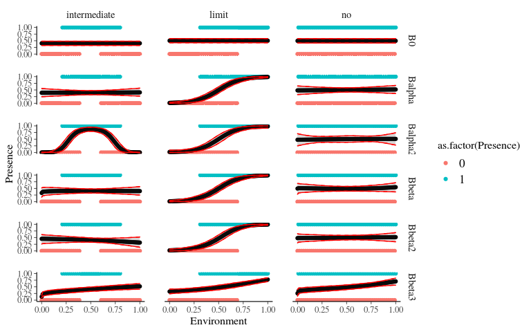
}Predictions
load("Wk7_save/SingleModel.Rdata")
g <- lapply(names(fits), function(model){
  lapply(as.list(names(data)), function(type)
    cbind(type = type, data[[type]],
          mu = apply(as.matrix(fits[[model]][[type]], pars = "theta"), 2, mean),
          t(apply(as.matrix(fits[[model]][[type]], pars = "theta"), 2,
                  quantile, probs = c(0.05, 0.95))))) %>%
    bind_rows() %>%
    mutate(model = model)
}) %>% bind_rows() %>%
  ggplot(aes(x = Environment)) +
  geom_point(aes(y = Presence, col = as.factor(Presence))) +
  geom_point(aes(y = mu)) +
  geom_ribbon(aes(ymin = `5%`, ymax = `95%`), color = 'red', alpha = 0.2) +
  geom_line(aes(y = `5%`), col = "red", alpha = 1, size = 0.5, linetype = "dashed") +
  geom_line(aes(y = `95%`), col = "red", alpha = 1, size = 0.5, linetype = "dashed") +
  facet_grid(model ~ type, scales = "free")
Predictions
Species joint distribution
Data
n <- 100
data <- list(
  no = data.frame(Environment = seq(0, 1, length.out = 100),
                  A = c(rep(0:1, 50)),
                  B = c(rep(c(1,0), 50)),
                  C = c(rep(c(1,0), 50))),
  intermediate = data.frame(Environment = seq(0, 1, length.out = n),
                            A = c(rep(0, 20),
                                  rep(0:1,10),
                                  rep(1,20),
                                  rep(0:1,10),
                                  rep(0,20)),
                            B = c(rep(0, 5),
                                  rep(0:1,10),
                                  rep(1,20),
                                  rep(0:1,10),
                                  rep(0,35)),
                            C = c(rep(0, 35),
                                  rep(0:1,10),
                                  rep(1,20),
                                  rep(0:1,10),
                                  rep(0,5))),
  limit = data.frame(Environment = seq(0, 1, length.out = n),
                     A = c(rep(0,30), rep(0:1,20), rep(1,30)),
                     B = c(rep(0, 20),
                           rep(0:1,10),
                           rep(1,20),
                           rep(0:1,10),
                           rep(0,20)),
                     C = c(rep(1,30), rep(0:1,20), rep(0,30)))
)
data <- lapply(data, function(x) x %>%
         reshape2::melt(id.vars = "Environment",
                        variable.name = "Species", value.name = "Presence") %>%
         filter(Presence != 0) %>%
         dplyr::select(-Presence))
mdata <- lapply(data, function(x)
  list(N = nrow(x),
       S = length(unique(x$Species)),
       K = 1,
       X = matrix(x$Environment),
       Y = sapply(levels(as.factor(x$Species)),
                  function(sp) as.numeric(x$Species == sp))))
Model
\[Presence \sim \mathcal{Dirichlet~Multinomial}(\\softmax(\alpha + \beta*E + \gamma*E^2))\]
\[LPMF(y|\alpha) = \Gamma(\sum \alpha) + \sum(\Gamma(\alpha + y)) \\- \Gamma(\sum \alpha+\sum y) - \sum\Gamma(\alpha)\]
Stan code - data
\[Presence \sim \mathcal{Dirichlet~Multinomial}(softmax(\alpha + \beta*E + \gamma*E^2))\]
data {
  int<lower = 1> N  ;       // # of individuals
  int<lower = 1> S  ;       // # of species
  int<lower = 1> K  ;       // # of environmental descriptors
  int<lower = 0, upper=1> Y[N, S]  ; // individuals presence or absence for each species
  matrix[N,K] X ;           // environmental descriptors
}
Stan code - parameters
\[Presence \sim \mathcal{Dirichlet~Multinomial}(softmax(\alpha + \beta*E + \gamma*E^2))\]
parameters {
  vector[S] alpha ; // intercept
  matrix[S,K] beta ; // sigmoidal slope
  matrix[S,K] gamma ; // quadratic form
}
Stan code - model
\[Presence \sim \mathcal{Dirichlet~Multinomial}(softmax(\alpha + \beta*E + \gamma*E^2))\]
model {
  alpha ~ normal(0,1) ;
  for(k in 1:K){
    beta[,k] ~ normal(0,1) ;
    gamma[,k] ~ normal(0,1) ;
  }
  for (n in 1:N)
    Y[n] ~ dirichlet_multinomial(softmax(alpha +
                                         beta*to_vector(X[n,]) +
                                         gamma*to_vector(X[n,] .* X[n,])))  ;
}
Stan code - LPMF
\[LPMF(y|\alpha) = \Gamma(\sum \alpha) + \sum(\Gamma(\alpha + y)) \\- \Gamma(\sum \alpha+\sum y) - \sum\Gamma(\alpha)\]
functions {
  real dirichlet_multinomial_lpmf(int[] y, vector alpha) {
    real alpha_plus = sum(alpha);
    return lgamma(alpha_plus) + sum(lgamma(alpha + to_vector(y)))
                - lgamma(alpha_plus+sum(y)) - sum(lgamma(alpha));
  }
}
Stan code - Full
functions {
real dirichlet_multinomial_lpmf(int[] y, vector alpha) {
real alpha_plus = sum(alpha);
return lgamma(alpha_plus) + sum(lgamma(alpha + to_vector(y)))
- lgamma(alpha_plus+sum(y)) - sum(lgamma(alpha));
}
}
data {
int<lower = 1> N ; // # of individuals
int<lower = 1> S ; // # of species
int<lower = 1> K ; // # of environmental descriptors
int<lower = 0, upper=1> Y[N, S] ; // individuals presence or absence for each species
matrix[N,K] X ; // environmental descriptors
}
parameters {
vector[S] alpha ; // intercept
matrix[S,K] beta ; // sigmoidal slope
matrix[S,K] gamma ; // quadratic form
}
model {
alpha ~ normal(0,1) ;
for(k in 1:K){
beta[,k] ~ normal(0,1) ;
gamma[,k] ~ normal(0,1) ;
}
for (n in 1:N)
Y[n] ~ dirichlet_multinomial(softmax(alpha +
beta*to_vector(X[n,]) +
gamma*to_vector(X[n,] .* X[n,]))) ;
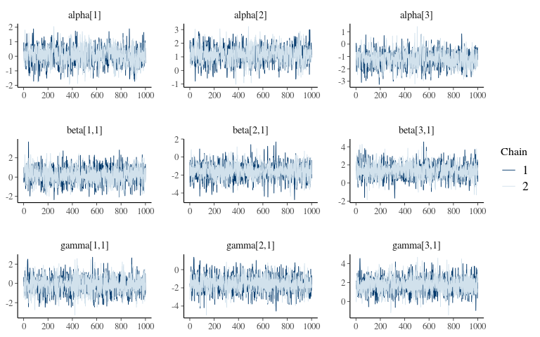
}Fit
Trace
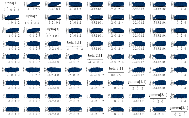
Pairs
Predictions
g <- lapply(names(mdata), function(type)
  lapply(1:3, function(sp)
    cbind(type = type, data[[type]],
          species = LETTERS[sp],
          Environment = data[[type]]$Environment,
          theta = apply(as.matrix(fits[[type]],
                                  pars = paste0("theta[", 1:mdata[[type]]$N, ",", sp, "]")),
                        2, mean),
          theta5 = apply(as.matrix(fits[[type]],
                                   pars = paste0("theta[", 1:mdata[[type]]$N, ",", sp, "]")),
                         2, quantile, probs = 0.05),
          theta95 = apply(as.matrix(fits[[type]],
                                    pars = paste0("theta[", 1:mdata[[type]]$N, ",", sp, "]")),
                          2, quantile, probs = 0.95))) %>%
  bind_rows()) %>%
  bind_rows() %>%
  ggplot(aes(x = Environment, col = species)) +
  geom_ribbon(aes(ymin = theta5, ymax = theta95), alpha = 0.2) +
  geom_line(aes(y = theta)) +
  facet_wrap(~ type, nrow = 3)
Predictions
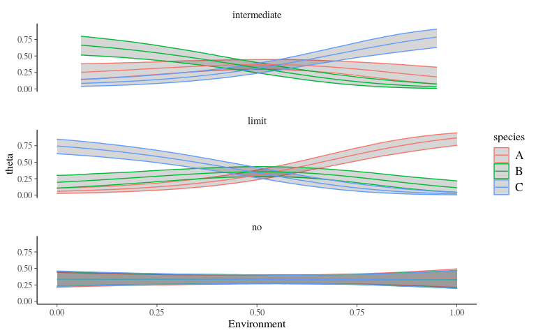
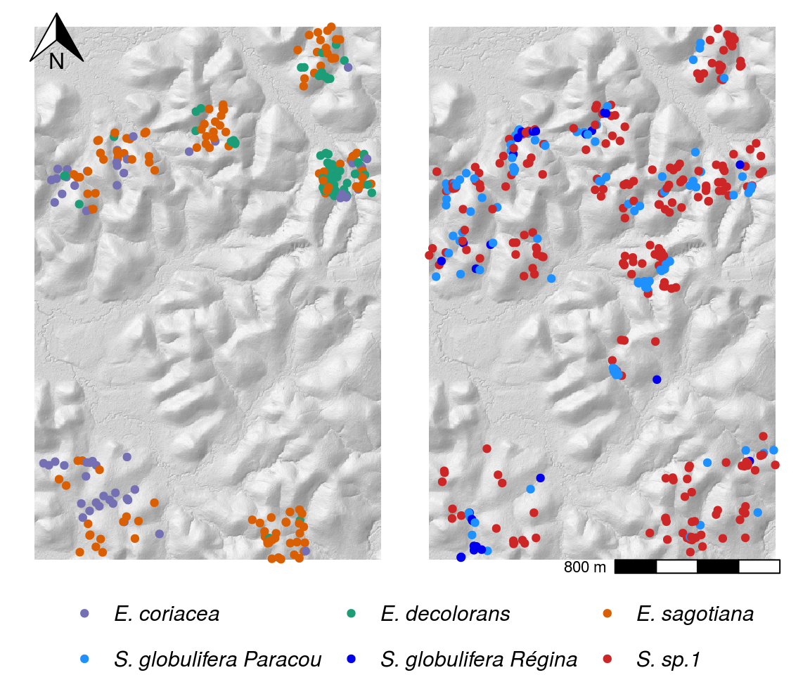
Species complexes in Paracou
Topographic Wetness Index
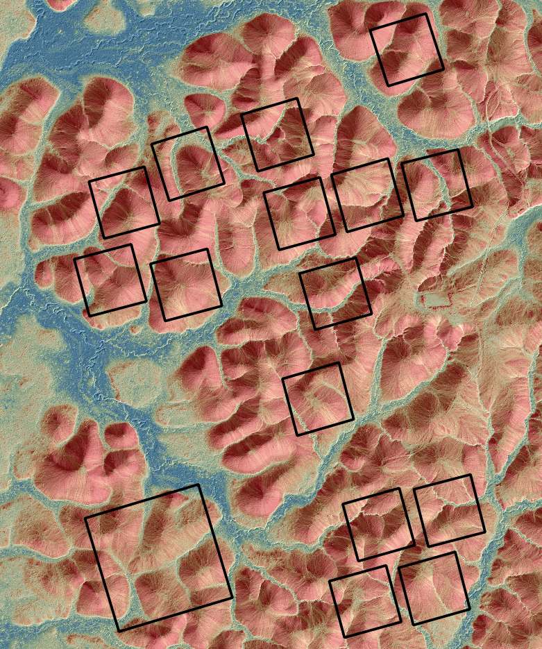
Topographic Wetness Index.
Neighbor Crowding Index
\[NCI_i = \sum _{j|\delta_{i,j}<20m} ^{J_i} DBH_j ^2 e^{-\frac{1}{4}\delta_{i,j}}\]
Posteriors
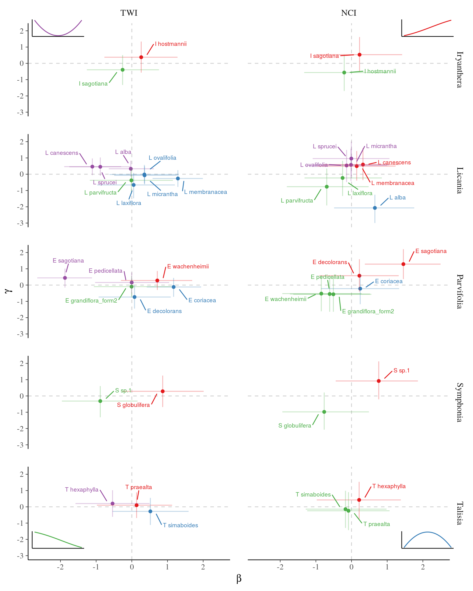
Posteriors.
Predictions
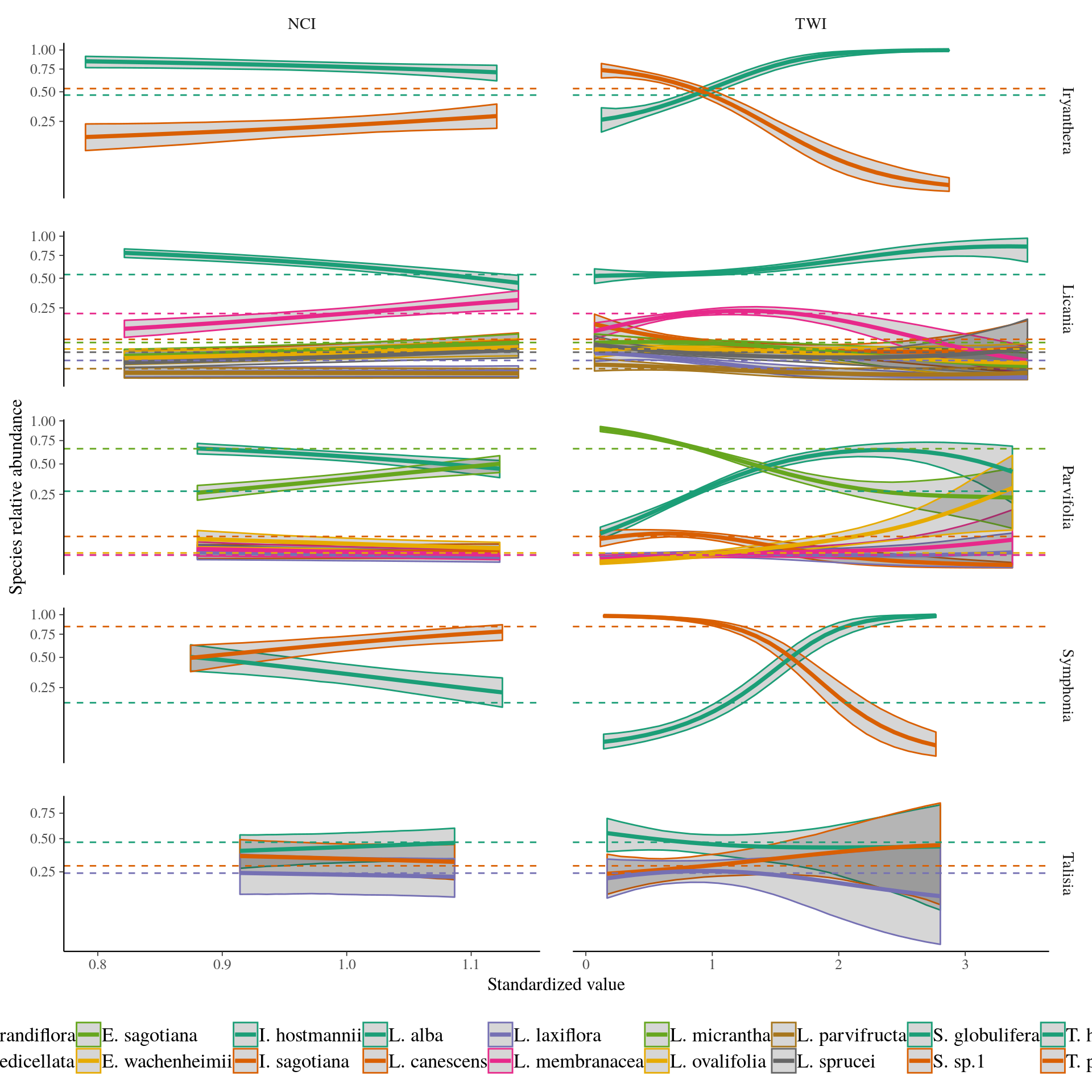
Predictions.